From "Trees Always Win" to Tabular Foundation Models
Why trees always won on tabular data — and what finally changed that.
You’re scrolling through Kaggle code. Reading a senior’s thesis. Browsing papers online. If the data sits in a table, one name shows up everywhere: XGBoost.
It’s the baseline nobody wants to face. Almost always wins. And when it does lose? Usually to another tree-based model.
Deep learning is incredible for images, text, audio. But tabular data? Different story.
This isn’t a myth. There’s a paper, “Why do tree-based models still outperform deep learning on typical tabular data?”, that tested this claim seriously: 45 datasets, various state-of-the-art deep learning models, compared head-to-head against XGBoost and Random Forest. The result? Tree-based models are still state-of-the-art, even before accounting for their training speed advantage.
But why? To answer that, we need to step back first.
To understand why trees are so hard to beat, we first need to look at what tabular data actually looks like in the real world, and why its nature makes neural networks struggle.
Most data used by organizations comes in tables. Patient records at hospitals, credit scores at banks, click logs on ad platforms, customer churn data. All tabular. And each dataset is always a mix: some columns are numerical, some categorical, some binary, with different scales and distributions in every column.
The problem isn’t just about the format. There’s something more fundamental: tabular data has no inherent structure between columns. Images have spatial structure, with nearby pixels related to each other. Text has sequential structure, where the order of words creates meaning. Tabular data has neither.
This is what’s known as inductive bias, the built-in assumptions about data shape that help a model learn more efficiently. CNNs are built on the assumption of spatial locality. Transformers are built on the assumption of sequential order. Both are effective precisely because there’s structure to exploit.
Tabular data has no such inductive bias. Column 3 and column 4 have no meaningful positional relationship. The relationships between features have to be learned from scratch, with no shortcuts. That’s a heavy burden, especially when data is limited.
Then there are the practical challenges. Real-world tabular datasets are rarely clean: missing values, noise, columns with mixed formats, numbers alongside text alongside dates. Out of hundreds of features, often only a small fraction are truly relevant. Everything, from normalizing values to encoding text as numbers to filling in missing data, has to be done manually before a model can even start training.
And preprocessing choices have real consequences. Take categorical feature encoding: one-hot encoding bloats the table with empty columns, while ordinal encoding creates an implicit ordering that wasn’t there before. Neither is always right, and small mistakes here can carry through to the final predictions.
Tree-based models don’t have these problems. The way they work is a natural fit for tabular data: they learn rules. For example: “If income > $50k and age < 60, the loan application is likely approved.” Decision trees are very good at finding conditional rules like this directly from data, without needing abstract representations. The splitting process automatically ignores uninformative features. Out of 100 columns, if only 10 are relevant, the tree focuses on those 10.
XGBoost takes this further. Trees are built sequentially. Each new tree corrects the mistakes of the previous one. The result is an accurate model that trains relatively quickly, requires no normalization, no special data format, and is naturally robust to outliers.
Many architectures have been tried for this domain: standard MLPs, TabNet (designed to automatically select relevant features), and transformer-based models like FT-Transformer. A survey, “Deep Neural Networks and Tabular Data: A Survey”, evaluating 11 deep learning approaches reached the same conclusion: gradient-boosted tree ensembles are still superior, even with extensive tuning.
Neural networks need structure to exploit. Tabular data doesn’t have it. It’s no surprise the domain has been called “the last unconquered castle” for deep learning.
The question is no longer whether deep learning loses here. That’s settled. What remains: is this because it’s truly impossible, or because the approach has been wrong all along?
Turns out the approach has been wrong. Not because there’s no good enough architecture, but because the underlying paradigm was off from the start.
To understand why, we need a short detour into something that emerged from the world of LLMs: in-context learning (ICL).
You’re probably already familiar. When you give GPT a few input-output examples inside a prompt, then ask about a new case, the model can answer without being retrained. That’s ICL. The model “learns” directly from the examples in front of it at that moment, without any parameters changing.
This is what makes ICL fundamentally different from standard supervised learning. Fine-tuning changes model weights. ICL doesn’t. The model observes patterns from the context examples, then makes predictions, much like how humans learn from analogy. Everything happens in a single read-through, no training involved.
The practical advantage is immediate: no need for large labeled datasets, no training infrastructure. Just provide relevant examples and the model follows the pattern.
But what’s more interesting isn’t ICL itself, it’s the explanation behind it. The paper “Transformers Can Do Bayesian Inference” argues that ICL can be understood as a process of Bayesian inference. The basic idea is this: before seeing any data, the model has a prior, a rough intuition about how likely different answers are. As examples come in, that intuition is updated into a posterior: a conclusion that has taken the new evidence into account.
A model trained across many different tasks implicitly builds intuition about common patterns in data, not memorizing but genuinely understanding. The more diverse the tasks it has seen, the sharper the intuition. And when given new examples, it doesn’t start from scratch. Instead, it adjusts its understanding based on the data in front of it.
This also explains why large model capabilities often appear to “emerge” suddenly. It’s not magic. It’s that the model has seen enough diverse patterns to know which are most likely correct.
There are limits, of course. If the type of data encountered is completely outside the model’s training experience, its predictions will go wrong. What’s more critical: giving it more examples will actually reinforce its confidence in the wrong answer. If the base intuition is off, every conclusion built on top of it will be off too.
The implication is direct: the quality of ICL depends on how well the intuition was built during training. And if that intuition can be designed explicitly, rather than left to emerge on its own, this mechanism can be taught to any domain, including tabular data.
If the quality of ICL depends on the model’s initial intuition, the next question is clear enough: can we define that intuition upfront? Not wait for the model to build it during training, but design it explicitly before any training begins.
That’s what Prior-Data Fitted Networks (PFNs) do. The premise is simple: if we can define what the “general shape” of datasets a model might encounter looks like, we can generate thousands of synthetic datasets matching that shape, then train a transformer to make accurate predictions on them.
The training process works like this: for each synthetic dataset that gets generated, part of it becomes the examples the model sees, and the rest becomes the questions it has to answer. The model learns: given data like this, what prediction makes the most sense? This process is repeated millions of times across different datasets, until the model understands the general patterns.
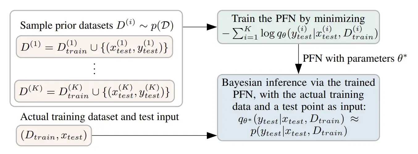
Train Once on Synthetic Data, Predict on Anything. Source: Transformers Can Do Bayesian Inference (2022).
The result is surprising. When given a real dataset it has never seen before, the model can make predictions immediately without any retraining, exactly like ICL in LLMs, but this time for supervised learning.
This proves something fairly important: we don’t need large amounts of real data to train a good model. As long as the synthetic data is representative enough, a model can learn from fabricated data and work directly in the real world. And the most natural domain to try first? Tabular data, precisely because we understand its structure the best.
A PFN designed specifically for tabular data — that’s TabPFN. Its first paper appeared at ICLR 2023, and it was the first time the PFN framework was applied directly to the tabular domain and tested head-to-head against trees.
TabPFN’s prior was designed to mimic the distribution of datasets that might exist in the real world. Its two main components are Bayesian Neural Networks and Structural Causal Models. The latter ensures that the synthetic datasets generated have plausible causal relationships between features, realistic noise, and diverse scales. One guiding principle: when two explanations are equally valid, prefer the simpler one.
Training happened once: a 12-layer Transformer trained for 20 hours on 8 GPUs. After that, the model was never retrained. When given a new dataset, just feed the training data as context. The model responds in a single forward pass, in under a second.
The results on 18 numerical datasets from OpenML-CC18 surprised many people. TabPFN outperformed XGBoost, LightGBM, and CatBoost, and matched the top AutoML systems given a full hour of tuning, with a large speed margin: 230× on CPU and 5,700× on GPU. Interestingly, TabPFN’s errors were weakly correlated with tree-based model errors, meaning the two often fail in different places. When combined in an ensemble, the result was better than either alone.
The results were also validated on 67 additional OpenML datasets with consistent findings. All code and trained models were released as open source with a scikit-learn interface. Just fit and predict. Community responses were mixed: some adopted it immediately, others were skeptical because the numbers seemed too good.
There are limits, of course. TabPFN v1 could only handle up to 1,000 rows, 100 numerical features, and 10 classes, with no missing values or categorical features. Beyond that, performance dropped. But the proof of concept worked: a transformer can learn to be an inference algorithm for tabular data and beat trees. This is where the term tabular foundation model was born.
Two years later, the second version arrived in Nature 2025. Same name, but far larger in scale. TabPFN v2 was trained on roughly 100 million synthetic datasets over two weeks, and this time could handle messier data: categorical features, missing values, outliers, and regression in addition to classification. The limits grew from 1,000 to 10,000 rows and from 100 to 500 features.
The architecture changed as well. V1 treated all data as a single token sequence. V2 has a dual attention mechanism that more explicitly exploits tabular structure: each cell attends to other features in its own row to understand row context, then attends to the same feature across all other rows to understand column context. The representation of each cell becomes rich from two directions at once. One additional benefit: if the training data doesn’t change, the computation can be cached and doesn’t need to be recomputed for each new prediction.
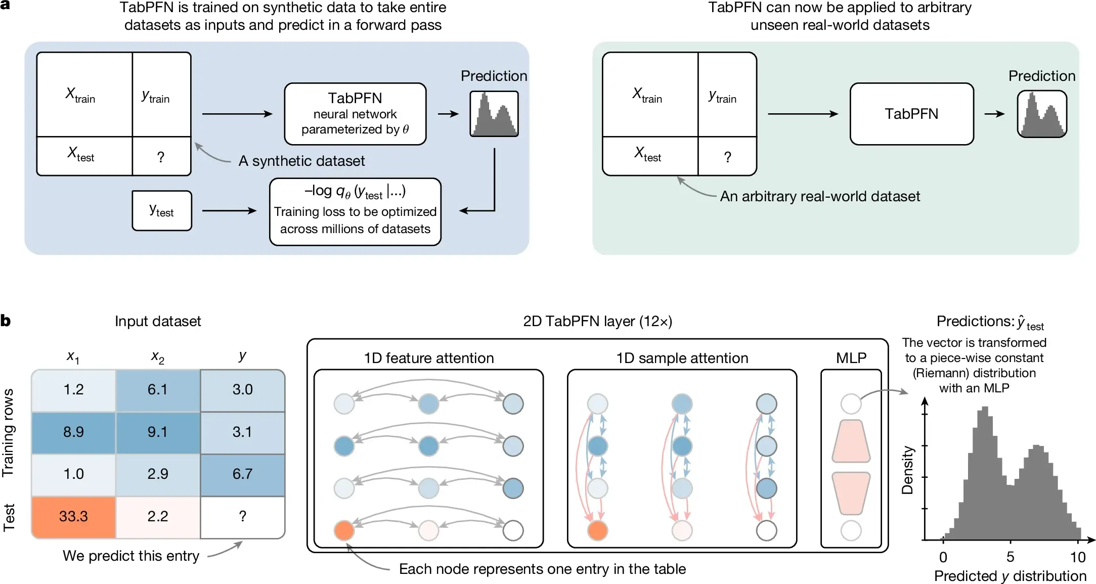
TabPFN v2 Architecture: Each Cell Attends to Its Row and Column. Source: Accurate predictions on small data with a tabular foundation model (2022).
In 2.8 seconds, TabPFN v2 outperformed CatBoost given 4 hours of tuning, with a 5,140× speedup for classification and 3,000× for regression. This paper was the first to use the term officially in its title: tabular foundation model.
Beyond raw performance, v2 gained capabilities that previously didn’t exist in any tabular model: fine-tuning support, synthetic data generation, probability distribution estimation, and reusable embeddings.
Adoption was fast. Within 10 months, the paper had nearly 400 citations and the open-source package had been downloaded over 2 million times. The medical field became the largest user, with more than 50 published applications, from cancer diagnosis to drug response prediction. Makes sense: TabPFN excels on small datasets, and medical data is rarely abundant.
The latest version, TabPFN-2.5, was released in November 2025 with capacity raised again, up to 50,000 rows and 2,000 features, 20 times larger than v2. There’s an interesting detail in its development: to find the best hyperparameter configuration, they used TabPFN v2 as a surrogate model. Literally, the new TabPFN was tuned by the old TabPFN. On small to medium datasets (≤10,000 rows), its win rate against default XGBoost reaches 100%. For larger datasets up to 100,000 rows, still 87%. If inference speed is a concern, a distillation feature can convert TabPFN into a standard MLP or tree ensemble ready for deployment.
A few years ago, the standard answer to beating trees on tabular data was always architecture. Build a transformer better suited for tables, add smarter regularization, or train on more real tabular datasets. The common approach was to force neural networks to work better on this kind of data.
TabPFN did none of that.
This model never saw a single real tabular dataset during training. Everything was done on synthetic data from the prior. At inference time there’s no gradient descent, no fitting. The model answers in a single forward pass. The way it works is more like performing inference from accumulated experience, not learning from scratch each time.
What was also unexpected was the decision boundary. Trees make decisions in a rigid way. One feature, one threshold, then split, resulting in box-shaped predictions in feature space. TabPFN produces predictions that are smoother, better calibrated, and better at capturing uncertainty. The two often fail in different places, which is exactly why combining them in an ensemble produces better results than either alone.
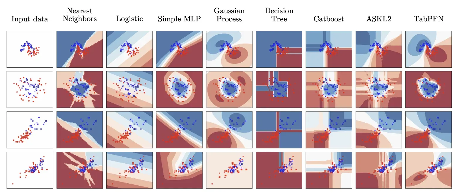
Decision Boundary: Trees vs TabPFN — Blocky vs Smooth. Source: TabPFN A Transformer That Solves Small Tabular Classification Problems in a Second (2022).
TabPFN also doesn’t rely on scale. No trillions of parameters, no massive datasets. With a 12-layer transformer trained for 20 hours, TabPFN v1 already outperformed AutoML given a full hour of tuning. Its success came not from size, but from how it represents the problem, and from a prior good enough to capture the diversity of real-world tabular data.
And maybe that’s the most unexpected lesson from this whole story. For domains where we can clearly define the structure, we don’t need to wait for large amounts of real data. Just define the prior correctly, generate synthetic data from it, and train a model to perform inference on top of it. Real data isn’t the only path.
XGBoost isn’t going anywhere. For large datasets, for production with tight latency requirements, for cases where interpretability is mandatory, trees are still a reasonable choice. TabPFN has its own limits. “Trees always win” is no longer an absolute truth, but that doesn’t mean trees have lost.
What changed is the question. Before: what architecture can beat trees on tabular data? Now: what prior best represents the distribution of datasets in your domain? That’s a more productive question, and a far more open one.
There’s a larger paradigm shift behind all this. For decades, we designed ML algorithms explicitly: define the architecture, choose the loss function, tune hyperparameters. TabPFN showed that the algorithm itself can be learned. Just define what “datasets that might exist in the world” look like, and let the model learn to be the best algorithm for that distribution.
For practitioners, the implication is straightforward. If you’re working with small to medium datasets and have GPU access, TabPFN is worth trying before jumping straight to XGBoost. Not because it’s always better, but because it’s zero-shot, no tuning required, no special preprocessing, and the results are often already very competitive. Its errors also differ from trees, making it easier to build effective ensembles.
And for me, still working through this for my thesis, the most memorable part isn’t the benchmark results. It’s realizing that the simple question “why do trees always win?” ends up opening a completely different way of thinking about machine learning.
- Why do tree-based models still outperform deep learning on typical tabular data? — Grinsztajn et al. (NeurIPS 2022)
- Deep Neural Networks and Tabular Data: A Survey — Borisov et al. (IEEE TNNLS 2024)
- Transformers Can Do Bayesian Inference — Müller et al. (ICLR 2022)
- TabPFN: A Transformer That Solves Small Tabular Classification Problems in a Second — Hollmann et al. (ICLR 2023)
- Accurate predictions on small data with a tabular foundation model — Hollmann et al. (Nature 2025)
- TabPFN-2.5: Advancing the State of the Art in Tabular Foundation Models — Grinsztajn et al. (arXiv 2025)